Test Functions for Bayesian Optimisation
Bayesian optimisation is a powerful optimisation technique for black-box functions and processes with expensive evaluations. It is popular for hyperparameter tuning in machine learning, but has many real-world applications as well.
At the centre of Bayesian optimisation is the objective function that we are trying to optimise. The objective function is usually expensive to evaluate, so before we start using Bayesian optimisation on the actual problem, we want to make sure that our code and models are working. In this post, we discuss a set of functions that can help us test and gauge the efficacy of our models. Along with the discussions are implementations in R.
library(ggplot2)
library(magrittr)
set.seed(4444)
set_dim <- `dim<-`Objective Functions in Bayesian Optimisation
The objective function or process, \(f(\mathbf{x})\), is a map from the input space \(\mathbf{x} \in \mathcal{X}\) to a scalar output \(y \in \mathbb{R}\):
\[f: \mathcal{X} \rightarrow \mathbb{R}\]
The true nature of this process is unknown and, for real world problems, might often be very difficult to traverse. A good set of test functions should challenge a model with different scenarios so we can gauge the strengths and weaknesses of our model.
An Example Model
In Bayesian optimisation, we model the objective function using a surrogate model, typically a Gaussian process (GP), which is cheap to evaluate and provides uncertainty estimates. Bayesian optimisation then uses an acquisition function to decide on the next point to evaluate in the search space.
To demonstrate the test functions we will implement a GP with an RBF kernel. For the acquisition function, we will use Expected Improvement (EI).
Show the code
#' RBF Kernel
#'
#' @param X1 matrix of dimensions (n, d). Vectors are coerced to (1, d).
#' @param X2 matrix of dimensions (m, d). Vectors are coerced to (1, d).
#' @param l length scale
#' @param sigma_f scale parameter
#'
#' @return matrix of dimensions (n, m)
rbf_kernel <- function(X1, X2, l = 1.0, sigma_f = 1.0) {
if (is.null(dim(X1))) dim(X1) <- c(1, length(X1))
if (is.null(dim(X2))) dim(X2) <- c(1, length(X2))
sqdist <- (- 2*(X1 %*% t(X2))) %>%
add(rowSums(X1**2, dims = 1)) %>%
sweep(2, rowSums(X2**2, dims = 1), `+`)
sigma_f**2 * exp(-0.5 / l**2 * sqdist)
}
#' Get Parameters of the Posterior Gaussian Process
#'
#' @param kernel kernel function used for the Gaussian process
#' @param X_pred matrix (m, d) of prediction points
#' @param X_train matrix (n, d) of training points
#' @param y_train column vector (n, d) of training observations
#' @param noise scalar of observation noise
#' @param ... named parameters for the kernel function
#'
#' @return list of mean (mu) and covariance (sigma) for the Gaussian
posterior <- function(kernel, X_pred, X_train, y_train, noise = 1e-8, ...) {
if (is.null(dim(X_pred))) dim(X_pred) <- c(length(X_pred), 1)
if (is.null(dim(X_train))) dim(X_train) <- c(length(X_train), 1)
if (is.null(dim(y_train))) dim(y_train) <- c(length(y_train), 1)
K <- kernel(X_train, X_train, ...) + noise**2 * diag(dim(X_train)[[1]])
K_s <- kernel(X_train, X_pred, ...)
K_ss <- kernel(X_pred, X_pred, ...) + 1e-8 * diag(dim(X_pred)[[1]])
K_inv <- solve(K)
mu <- (t(K_s) %*% K_inv) %*% y_train
sigma <- K_ss - (t(K_s) %*% K_inv) %*% K_s
list(mu = mu, sigma = sigma)
}
#' Gaussian Negative log-Likelihood of a Kernel
#'
#' @param kernel kernel function
#' @param X_train matrix (n, d) of training points
#' @param y_train column vector (n, d) of training observations
#' @param noise scalar of observation noise
#'
#' @return function with kernel parameters as input and negative log likelihood
#' as output
nll <- function(kernel, X_train, y_train, noise) {
function(params) {
n <- dim(X_train)[[1]]
K <- rlang::exec(kernel, X1 = X_train, X2 = X_train, !!!params)
L <- chol(K + noise**2 * diag(n))
a <- backsolve(r = L, x = forwardsolve(l = t(L), x = y_train))
0.5*t(y_train)%*%a + sum(log(diag(L))) + 0.5*n*log(2*pi)
}
}
#' Gaussian Process Regression
#'
#' @param kernel kernel function
#' @param X_train matrix (n, d) of training points
#' @param y_train column vector (n, d) of training observations
#' @param noise scalar of observation noise
#' @param ... parameters of the kernel function with initial guesses. Due to the
#' optimiser used, all parameters must be given and the order unfortunately
#' matters
#'
#' @return function that takes a matrix of prediction points as input and
#' returns the posterior predictive distribution for the output
gpr <- function(kernel, X_train, y_train, noise = 1e-8, ...) {
kernel_nll <- nll(kernel, X_train, y_train, noise)
param <- list(...)
opt <- optim(par = rep(1, length(param)), fn = kernel_nll)
opt_param <- opt$par
function(X_pred) {
post <- rlang::exec(
posterior,
kernel = kernel,
X_pred = X_pred,
X_train = X_train,
y_train = y_train,
noise = noise,
!!!opt_param
)
list(
mu = post$mu,
sigma = diag(post$sigma),
Sigma = post$sigma,
parameters = set_names(opt_param, names(param))
)
}
}
#' Expected Improvement Acquisition Function for a Gaussian Surrogate
#'
#' @param mu vector of length m. Mean of a Gaussian process at m points.
#' @param sigma vector of length m. The diagonal of the covariance matrix of a
#' Gaussian process evaluated at m points.
#' @param y_best scalar. Best mean prediction so far on observed points
#' @param xi scalar, exploration/exploitation trade off
#' @param task one of "max" or "min", indicating the optimisation problem
#'
#' @return EI, vector of length m
expected_improvement <- function(mu, sigma, y_best, xi = 0.01, task = "min") {
if (task == "min") imp <- y_best - mu - xi
if (task == "max") imp <- mu - y_best - xi
if (is.null(imp)) stop('task must be "min" or "max"')
Z <- imp / sigma
ei <- imp * pnorm(Z) + sigma * dnorm(Z)
ei[sigma == 0.0] <- 0.0
ei
}
#' Plot of a Gaussian Process in One Dimension
#'
#' @param mu vector of length m. Mean of a Gaussian process at m points.
#' @param sigma vector of length m. The diagonal of the covariance matrix of a
#' Gaussian process evaluated at m points.
#' @param X_pred matrix of dimensions (m X 1) representing m prediction points
#' with one dimension.
#' @param X_train matrix of dimensions (n X 1) representing n training points
#' with one dimension
#' @param y_train vector of length n representing n observations at points
#' X_train
#' @param true_function function representing the objective function (in real
#' life, this function is unknown and cannot be plotted)
#'
#' @return ggplot2 plot
gp_1d_plot <- function(mu, sigma, X_pred, X_train, y_train, true_function) {
tibble::tibble(
m = mu,
uncertainty = 1.96*sqrt(sigma),
upper = m + uncertainty,
lower = m - uncertainty,
x = X_pred,
f = true_function(X_pred)
) %>%
ggplot(aes(x = x)) +
geom_line(aes(y = m, colour = "Mean")) +
geom_ribbon(
aes(ymin = lower, ymax = upper, fill = "89% interval"),
alpha = 0.2
) +
geom_point(
data = tibble::tibble(x = X_train, y = y_train),
aes(x = x, y = y, shape = "Training point"),
colour = "#fb8500",
size = 4
) +
geom_line(mapping = aes(y = f, colour = "True function")) +
scale_shape_manual(values = c("Training point" = "+")) +
scale_fill_manual(values = c("89% interval" = "#219ebc")) +
labs(shape = "") +
theme_minimal() +
labs(
y = "y",
x = "",
colour = "",
fill = ""
) +
theme(panel.grid = element_blank(), axis.text.x = element_blank())
}
#' Plot of Acquisition Function with Surrogate in One Dimension
#'
#' @X_pred matrix of dimensions (m X 1) representing m prediction points with
#' one dimension.
#' @acquisition_function vector of length m representing the acquisition
#' function evaluated at the m points of X_pred
#' @param uncertainty_plot the plot of a surrogate model in one dimension
#' @param xt1 scalar, the point, x, that optimises the acquisition function
#' @param label character, label for the acquisition function
#' @param title character, a title for the plot
#'
#' @return ggplot2 plot
acquisition_plot <- function(X_pred,
acquisition_function,
uncertainty_plot,
xt1,
label = "EI",
title = "") {
p1 <- tibble::tibble(
x = X_pred,
a = acquisition_function
) %>%
ggplot() +
geom_line(aes(x = x, y = a, colour = label)) +
geom_vline(xintercept = xt1, linetype = 2) +
theme_minimal() +
labs(x = "", y = label, colour = "") +
theme(panel.grid = element_blank())
p2 <- uncertainty_plot +
geom_vline(xintercept = xt1, linetype = 2) +
labs(title = title)
aligned_plots <- cowplot::align_plots(p2, p1 , align = "v")
cowplot::plot_grid(aligned_plots[[1]], aligned_plots[[2]], ncol = 1)
}
gp_rbf_ei_1d <- function(X_train,
X_pred,
demo_function,
noise = 1e-8,
title = "" ) {
y_train <- demo_function(X_train) + rnorm(nrow(X_train), 0, noise)
gp <- gpr(
kernel = rbf_kernel,
X_train = X_train,
y_train = y_train,
noise = noise,
l = 1,
sigma_f = 1
)
post_pred <- gp(X_pred)
mu <- post_pred$mu
sigma <- post_pred$sigma
ei <- expected_improvement(mu = mu, sigma = sigma, y_best = min(y_train))
gp_plot <- gp_1d_plot(
mu = mu,
sigma = sigma,
X_pred = X_pred,
X_train = X_train,
y_train = y_train,
true_function = demo_function
)
acquisition_plot(
X_pred = X_pred,
acquisition_function = ei,
uncertainty_plot = gp_plot,
xt1 = X_pred[which.max(ei)],
label = "EI",
title = paste("Gaussian Process Surrogate", title)
)
}For each test function, we will condition the GP on a set of six training points. Here is an example applied to a simple function:
demo_objective_function <- function(x) sin(12 * x) * x + 0.5 * x^2
X_train <- matrix(c(0.02, 0.3, 0.55, 0.75, 0.8, 0.98), 6, 1)
noise <- 0.05
y_train <- demo_objective_function(X_train) + rnorm(6, 0, noise)
X_pred <- matrix(seq(0, 1, length.out = 100), 100, 1)
gp_rbf_ei_1d(
X_train = X_train,
X_pred = X_pred,
demo_function = demo_objective_function,
noise = noise
)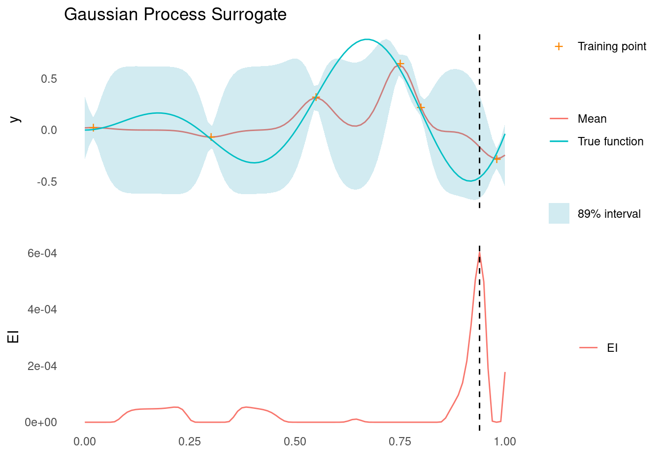
The vertical dashed line indicates the next point that would be evaluated in our hypothetical Bayesian optimisation scenario.
Test Functions with Continuous Dimensions
We start out with test functions that are defined for any number, \(d\) of continuous dimensions.
When doing Bayesian optimisation, it is prudent to normalise the input dimensions such that the search space is confined to the unit hypercube:
\[\mathcal{X} = [0,1]^d\]
Most of the following functions are not defined in the unit hypercube, however. So along with each function, we also define a scaling function to scale the input dimensions from the unit hypercube to the range of the function.
Before we get started, we define a nice surface plot to visualise each function.
Show the code
surface_plot_2d <- function(fun, scale) {
n <- 300
x <- scale(seq(0, 1, length.out = n))
y <- expand.grid(x , x) %>%
fun() %>%
set_dim(c(n, n))
plotly::plot_ly(
x = x,
y = x,
z = y,
showscale = FALSE
) %>%
plotly::add_surface(
contours = list(
z = list(
show = TRUE,
start = min(y),
end = max(y),
size = (max(y) - min(y)) / 15,
color = "white",
usecolormap = TRUE,
highlightcolor = "#ff0000",
project = list(z = TRUE)
)
)
) %>%
plotly::layout(
plot_bgcolor = "rgba(0,0,0,0)",
paper_bgcolor = "rgba(0,0,0,0)",
scene = list(camera = list(eye = list(x = 2.2, y = 1.8, z = 1.5)))
)
}Ackley
There are several Ackley test functions, one of them is defined as [1]:
\[ \begin{array}{cc} f(\mathbf{x}) = & -20\exp\left(-0.2\sqrt{\frac{1}{d}\sum_{i=1}^dx_i^2}\right) \\ & - \exp\left(\frac{1}{d}\sum_{i=1}^d \cos(2\pi x_i)\right) \\ & + 20 + \exp(1) \end{array} \]
where \(d\) is the number of dimensions. Sometimes the function is defined with adjustable parameters in place of the constants, but the constants used here appear often [2].
ackley <- function(X) {
if (is.null(dim(X))) set_dim(X, c(1, length(X)))
d <- ncol(X)
part1 <- -20 * exp(-0.2 * sqrt(1 / d * rowSums(X^2)))
part2 <- -exp(1 / d * rowSums(cos(2 * pi * X)))
part1 + part2 + 20 + exp(1)
}\(\mathbf{x}\) is limited to \(-35 > x_i < 35\), though the range \(-5 < x_i < 5\) is plenty challenging. The global minimum of the Ackley function is \(f(\mathbf{x})=0\) at \(\mathbf{x}=(0,0,...,0)\).
Show the code
ackley_scale <- function(X) X * 10 - 5
surface_plot_2d(ackley, ackley_scale)When conditioning a GP with an RBF kernel on the 1D Ackley function, the global trend is fairly easily captured. However, the local periodic component is not captured. The use of a periodic kernel along with the RBF kernel would possibly remedy that, but it is not necessary when we are looking for the global minimum.
gp_rbf_ei_1d(
X_train = ackley_scale(X_train),
X_pred = ackley_scale(X_pred),
demo_function = ackley,
noise = 0.4,
title = "on the 1D Ackley Function"
)
Michalewicz
The Michalewicz test function defined as [1]:
\[f(\mathbf{x}) = -\sum_{i = 1}^d\sin(x_i)\sin^{2m}\left(\frac{ix_i^2}{\pi}\right)\]
where \(m\) is a constant commonly set to 10.
michalewicz <- function(X, m = 10) {
i <- seq_len(dim(X)[[2]]) / pi
s <- t(i * t(X**2))
- rowSums(sin(X) * sin(s)**(2 * m))
}The function is usually evaluated in the range \(x_i \in [0, \pi]\) for all dimensions.
The Michalewicz test function features large swaths of space with virtually no gradient, making it very hard to optimise unless a training point happens to be close to the global optimum.
Show the code
michalewicz_scale <- function(X) X * pi
surface_plot_2d(michalewicz, michalewicz_scale)The elusiveness of the global optimum is only exacerbated in higher dimensions. The location and value of the global minimum depends on the number of dimensions, but in two dimensions it is [3]:
\[f(x_1 = 2.20, x_2 = 1.57) \approx -1.80\]
It is difficult to capture the overall trend of the Michalewicz function with a GP, even in 1D. Unless a training point happens to be close to the optimum, there is very little information to go on. When looking at the uncertainties reported by the GP, this results in an almost uniform band along the main plane of the function.
gp_rbf_ei_1d(
X_train = michalewicz_scale(X_train),
X_pred = michalewicz_scale(X_pred),
demo_function = michalewicz,
noise = 0.05,
title = "on the 1D Michalewicz Function"
)
Rastrigin
The Rastrigin function is defined as [3]:
\[f(\mathbf{x}) = 10d + \sum_{i=1}^dx_i^2-10\cos(2\pi x_i)\]
rastrigin <- function(X) 10 * dim(X)[[2]] + rowSums(X^2 - 10 * cos(2 * pi * X))The usual evaluation range is \(-5.12 < x_i < 5.12\).
The function is essentially a large bowl shape with a periodic element that causes the function to have many local minima. The global minimum of th Rastrigin function is \(f(\mathbf{x})=0\) at \(\mathbf{x}=(0,0,...,0)\).
Show the code
rastrigin_scale <- function(X) X * 10.24 - 5.12
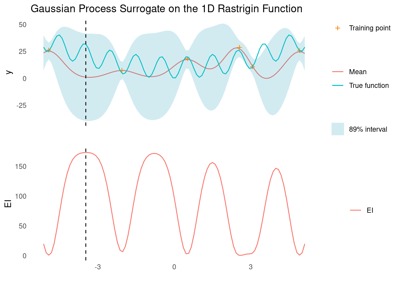
surface_plot_2d(rastrigin, rastrigin_scale)Like for the Ackley function, a GP with an RBF kernel is incapable of capturing the periodic element of the test function but is enough for capturing the large scale trend, which is sufficient to find the global optimum. Bayesian optimisation is hampered by the deep local minima though.
gp_rbf_ei_1d(
X_train = rastrigin_scale(X_train),
X_pred = rastrigin_scale(X_pred),
demo_function = rastrigin,
noise = 4,
title = "on the 1D Rastrigin Function"
)
Styblinski-Tang
The Styblinski-Tang function is defined as [1]:
\[f(\mathbf{x}) = 0.5\sum_{i=1}^dx_i^4-16x_i^2+5x_i\]
styblinski_tang <- function(X) 0.5 * rowSums(X^4 - 16 * X^2 + 5 * X)The usual evaluation range is \(-5 < x_i < 5\) for all dimensions and the global minimum is \(f(\mathbf{x}) = -39.17d\) for \(x_i = -2.903534\) in all dimensions.
The function is a large bowl with multiple local minima that are close in absolute value to the global minimum.
Show the code
styblinski_tang_scale <- function(X) X * 10 - 5
surface_plot_2d(styblinski_tang, styblinski_tang_scale)A GP with an RBF kernel makes quick work of the Styblinski-Tang function, and we should be able to find the global minimum with just a few evaluations in 1D.
gp_rbf_ei_1d(
X_train = styblinski_tang_scale(X_train),
X_pred = styblinski_tang_scale(X_pred),
demo_function = styblinski_tang,
noise = 4,
title = "on the 1D Styblinski-Tang Function"
)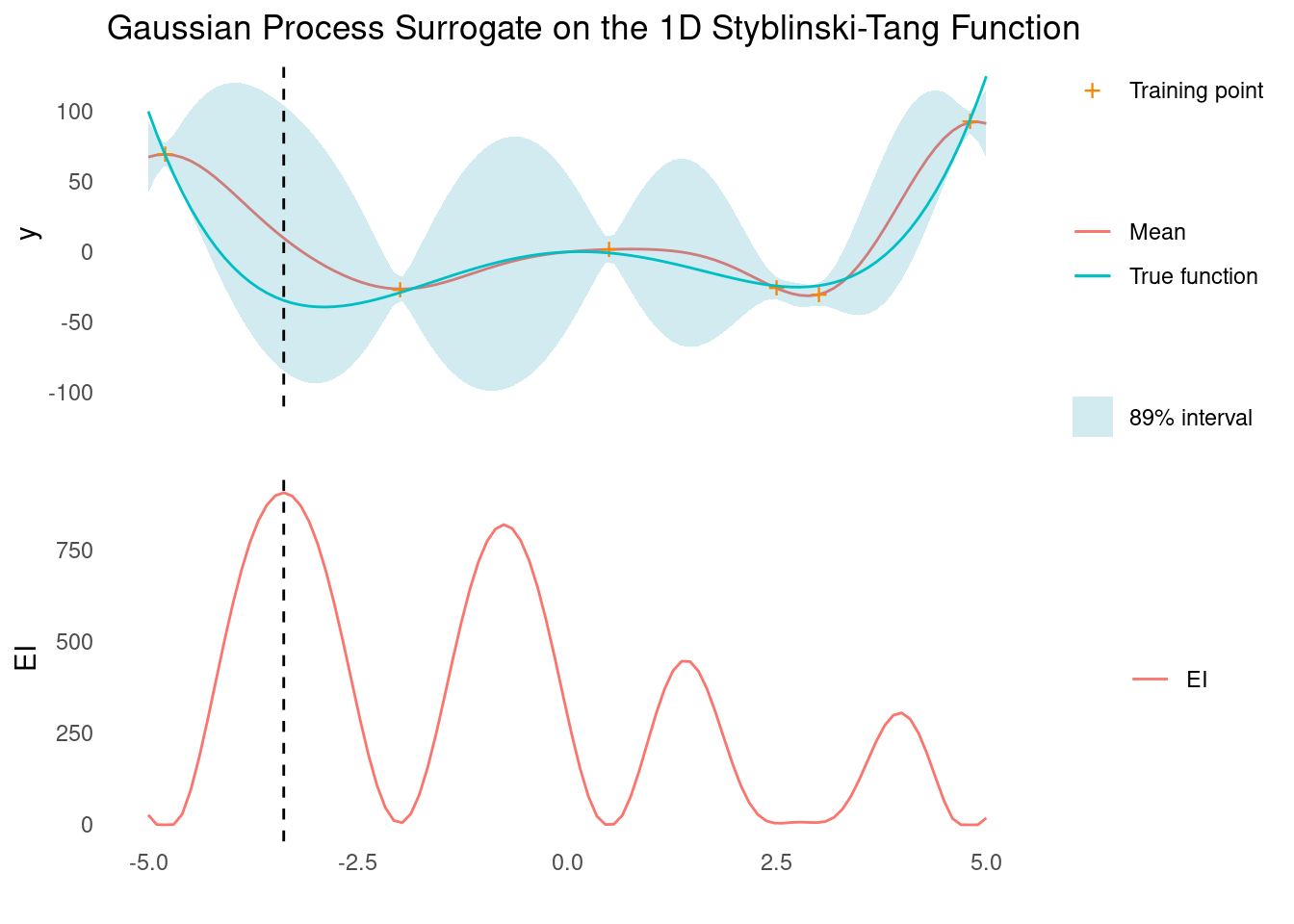
Note how the next evaluation would have yielded the global minimum.
Zakharov
The Zakharov function is defined as [1]:
\[f(\mathbf{x}) = \sum_{i=1}^d\left(x_i^2\right) + \left(\sum_{i=1}^d0.5ix_i\right)^2+ \left(\sum_{i=1}^d0.5ix_i\right)^4\]
zakharov <- function(X) {
sum_ix <- rowSums(t(t(X) + dim(X)[[2]]))
rowSums(X^2) + sum_ix^2 + sum_ix^4
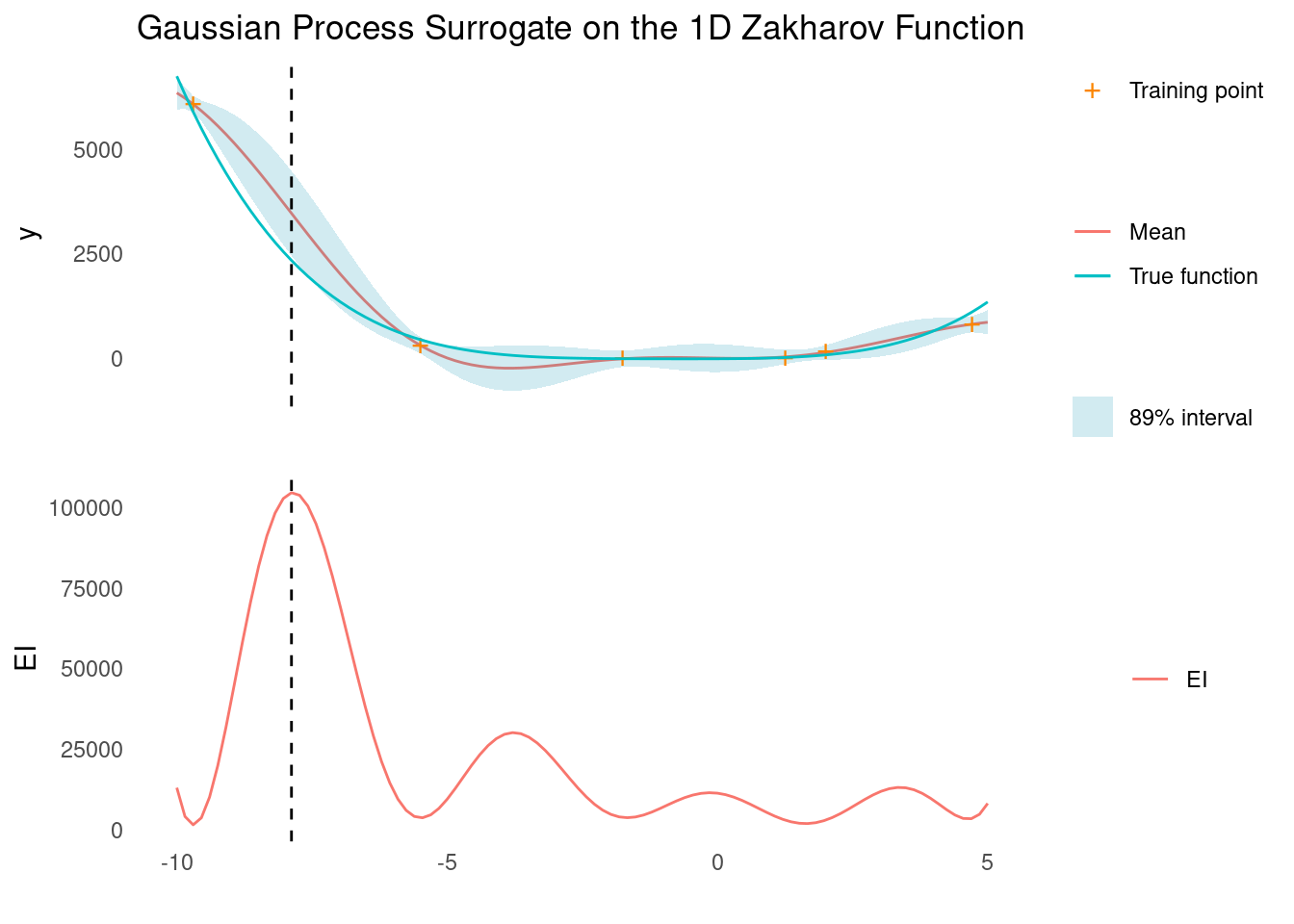
}The usual evaluation range is \(-5 < x_i < 10\) for all dimensions and the global minimum is \(f(\mathbf{x}) = 0\) for \(x_i = 0\) in all dimensions.
The function is a bent plane that has a very small derivative close to the global minimum.
Show the code
zakharov_scale <- function(X) X * 15 - 10
surface_plot_2d(zakharov, zakharov_scale)Despite the relatively simple looks of the function, it is very difficult for our GP with an RBF kernel to find the global minimum, even in 1D. This is because the RBF kernel is stationary, and the Zakharov function has vastly different length scales for different areas of search space. Combining the RBF kernel with a non-stationary kernel could probably remedy that.
gp_rbf_ei_1d(
X_train = zakharov_scale(X_train),
X_pred = zakharov_scale(X_pred),
demo_function = zakharov,
noise = 100,
title = "on the 1D Zakharov Function"
)
Test Functions in 2D
While it is rare to have a real world problem that features exactly two input dimensions, limiting ourselves to just two continuous inputs allows us to employ some quite difficult test functions.
Langermann
The Langermann functions is defined as [2]:
\[f(\mathbf{x}) = \sum_{j=1}^5c_j\exp\left(-\frac{1}{\pi}\sum_{i=1}^d\left(x_i-A_{ij}\right)^2\right)\cos\left(\pi\sum_{i=1}^d\left(x_i-A_{ij}\right)^2\right)\]
Where \(\mathbf{c} = [1, 2, 5, 2, 3]\) and
\[ \mathbf{A} = \left[\begin{array}{ccc} 3 & 5 \\ 5 & 2 \\ 2 & 1 \\ 1 & 4 \\ 7 & 9 \end{array}\right] \]
langermann <- function(X) {
d <- dim(X)[[2]]
cvec <- c(1, 2, 5, 2, 3)
A <- matrix(c(3, 5, 2, 1, 7, 5, 2, 1, 4, 9)[1:(d * 5)], nrow = 5)
purrr::map(1:5, function(j) {
xa <- rowSums(t(t(X) - A[j,])^2)
cvec[[j]] * exp((-1 / pi) * xa) * cos(pi * xa)
}) %>%
do.call(cbind, .) %>%
rowSums()
}The usual evaluation range is \(0 < x_i < 10\) for each dimension and the global minimum is \(f(\mathbf{x}) = 0\) for \(x_i = 0\) in all dimensions.
The function features a very diverse landscape with many local minima as well as areas with relatively small gradients.
Show the code
langermann_scale <- function(X) X * 10
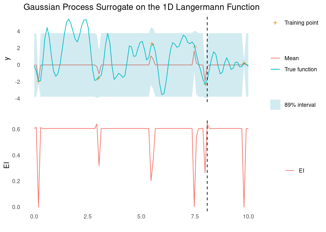
surface_plot_2d(langermann, langermann_scale)It is very difficult for a GP with an RBF kernel to capture the structure of the Langerman function, even in 1D. Given a small budget for training points, the best we can hope for is a good local minimum.
gp_rbf_ei_1d(
X_train = langermann_scale(X_train),
X_pred = langermann_scale(X_pred),
demo_function = langermann,
noise = 0.1,
title = "on the 1D Langermann Function"
)
Shubert
The Shubert function is defined as [2]:
\[\sum_{j=1}^5\cos\left((j+1)x_1+j\right)\cos\left((j+1)x_2+j\right)\]
The function is easily extended to any number of \(d\) dimensions [1] [3], and the implementation below reflects that. However, given the product across dimensions, the function may be numerically challenged in higher dimensions.
shubert <- function(X) {
purrr::map(1:5, ~ .x*cos((.x + 1) * X + .x)) %>%
purrr::reduce(`+`) %>%
apply(1, prod)
}The usual range of evaluation is \(-10 < x_i < 10\) for all dimensions.
The function features multiple global minima at \(f(\mathbf{x}) = −186.73\). I 2D there are 18 of them in the evaluation range.
Show the code
shubert_scale <- function(X) X*20 - 10
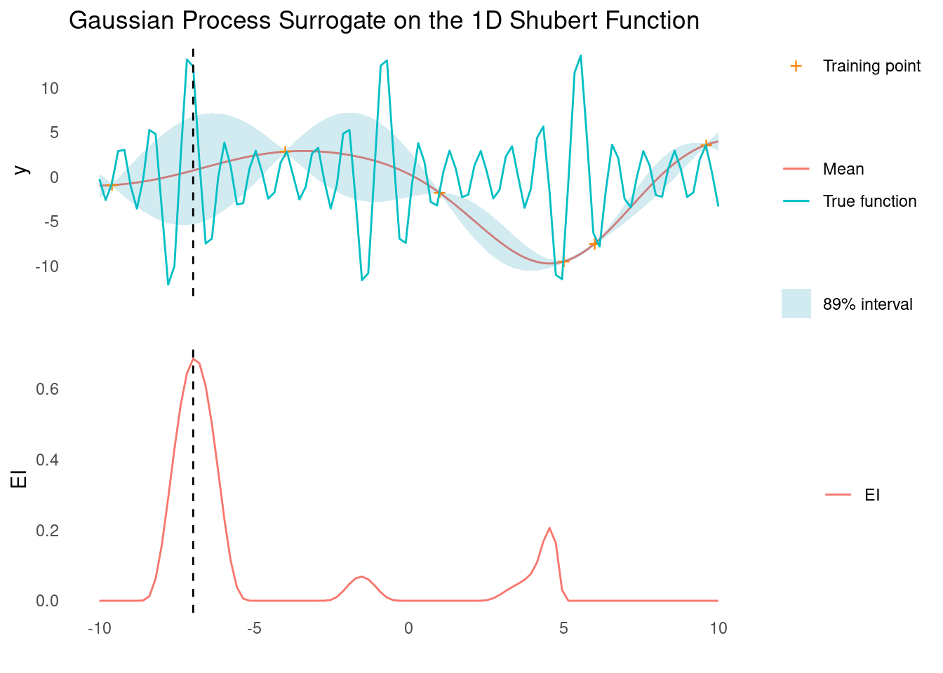
surface_plot_2d(shubert, shubert_scale)The Shubert function features periodic elements at different scales, which an RBF kernel cannot model. In 1D, Bayesian optimisation using a GP with an RBF kernel will probably still find a global minimum fairly quickly, however.
gp_rbf_ei_1d(
X_train = shubert_scale(X_train),
X_pred = shubert_scale(X_pred),
demo_function = shubert,
noise = 0.1,
title = "on the 1D Shubert Function"
)
References
License
The content of this project itself is licensed under the Creative Commons Attribution-ShareAlike 4.0 International license, and the underlying code is licensed under the GNU General Public License v3.0 license.
Anders E. Nielsen
Data Professional & Research Scientist
I apply modern data technology to solve real-world problems. My interests include statistics, machine learning, computational biology, and IoT.